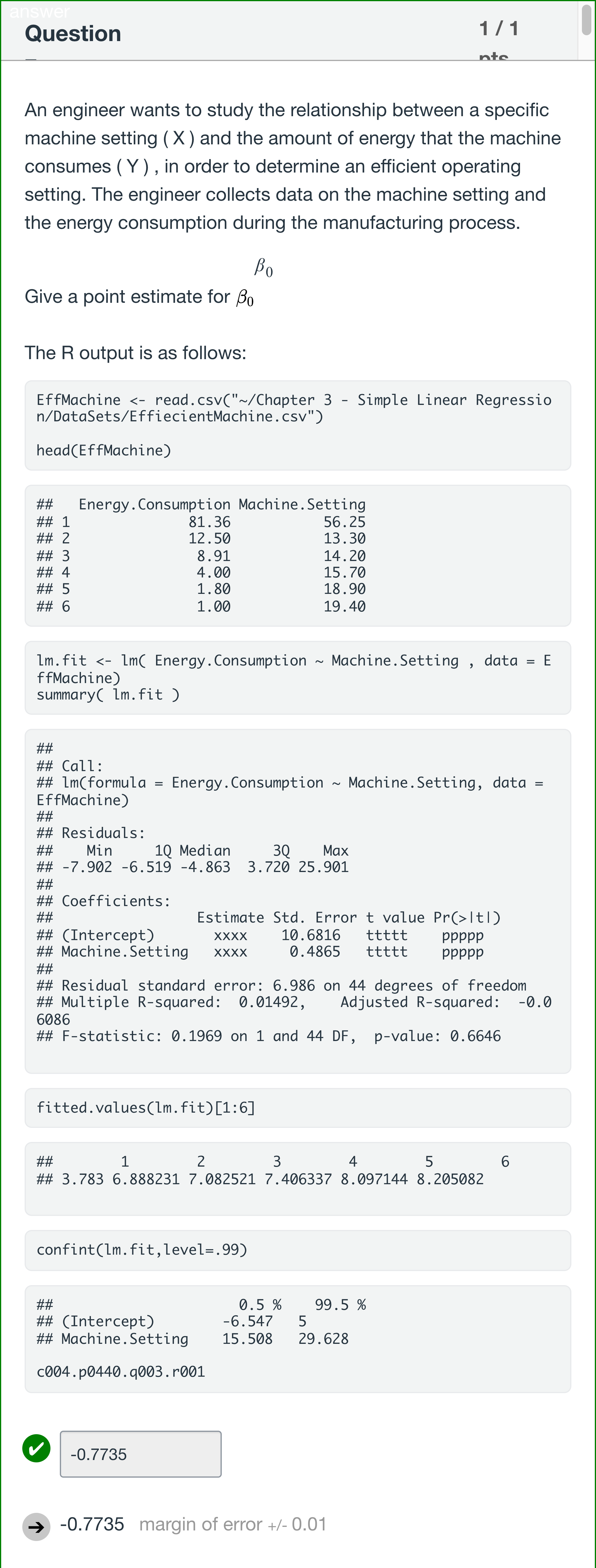
An engineer wants to study the relationship between a specific machine setting ( X ) and the amount of energy that the machine consumes ( Y ) , in order to determine an efficient operating setting. The engineer collects data on the machine setting and the energy consumption during the manufacturing process. Give a point estimate for     The R output is as follows: EffMachine <- read.csv("~/Chapter 3 - Simple Linear Regression/DataSets/EffiecientMachine.csv") head(EffMachine) ## Energy.Consumption Machine.Setting ## 1 81.36 56.25 ## 2 12.50 13.30 ## 3 8.91 14.20 ## 4 4.00 15.70 ## 5 1.80 18.90 ## 6 1.00 19.40 lm.fit <- lm( Energy.Consumption ~ Machine.Setting , data = EffMachine) summary( lm.fit ) ## ## Call: ## lm(formula = Energy.Consumption ~ Machine.Setting, data = EffMachine) ## ## Residuals: ## Min 1Q Median 3Q Max ## -7.902 -6.519 -4.863 3.720 25.901 ## ## Coefficients: ## Estimate Std. Error t value Pr(>|t|) ## (Intercept) xxxx 10.6816 ttttt ppppp ## Machine.Setting xxxx 0.4865 ttttt ppppp ## ## Residual standard error: 6.986 on 44 degrees of freedom ## Multiple R-squared: 0.01492, Adjusted R-squared: -0.06086 ## F-statistic: 0.1969 on 1 and 44 DF, p-value: 0.6646 fitted.values(lm.fit)[1:6] ## 1 2 3 4 5 6 ## 3.783 6.888231 7.082521 7.406337 8.097144 8.205082 confint(lm.fit,level=.99) ## 0.5 % 99.5 % ## (Intercept) -6.547 5 ## Machine.Setting 15.508 29.628 c004.p0440.q003.r001Short answer